1 Introduction
The simplest way to estimate a power spectral density (PSD) is to use a periodogram, defined as
periodogram <- function(x) (1/length(x))*abs(fft(x))^2where x is the data samples. The periodogram estimates the power level at \(N\) frequency locations where \(N\) is the number of samples in x. The periodogram uses \(N\) data samples to estimate \(N\) power levels. This leads to high variance estimates. There are ways to reduce the variance, but they also reduce the resolution.
A different approach is to estimate the PSD using a model. A good model can capture the important features of the PSD and be controlled by a few parameters. The autoregressive moving average (ARMA) model and the closely related autoregressive (AR) and moving average (MA) models can model a wide variety of PSDs and can be controlled by a few parameters.
This article defines the ARMA, AR, and MA models and then shows how to calculate their PSDs. We then cover how they are used to estimate PSDs, how to select between the three models, and how to choose the number of parameters (the model order). By the end of this article, you will understand how ARMA/AR/MA models are used for PSD estimation.
Much of this article comes from Chapter 8 of Power Spectral Density Estimation by Example Carbone (2022).
2 ARMA Model
An ARMA model of order \(p\), \(q\) is defined as
\[ a[0]y[n] = -\sum_{k=1}^p a[k]y[n-k] +\sum_{k=0}^q b[k]x[n-k], \tag{1}\]
where \(y[n]\) is the current output, \(a[k]\) and \(b[k]\) are the coefficients of the model, \(p\) is the number of \(a\) coefficients, \(q\) is number of \(b\) coefficients, \(y[n − k]\) are the past outputs, and \(x[n − k]\) are past (and present) inputs. The coefficient \(a[0]\) is always assumed to be 1, so from here on; we replace \(a[0]\) with 1. If \(a[k]\) \(\neq\) 1 we could divide Equation 1 by \(a[0]\).
The input \(x\) is a sequence of samples from a white noise process with variance \(\sigma^2\). The input process could be any white noise process, but for the sake of specificity, we assume the process is white Gaussian noise (WGN). The ARMA model of order \(p\), \(q\) is written as ARMA[\(p,q\)]. The parameters of the ARMA model are the autoregressive coefficients \(a[k]\), the moving average coefficients \(b[k]\), and the variance of the input \(\sigma^2\).
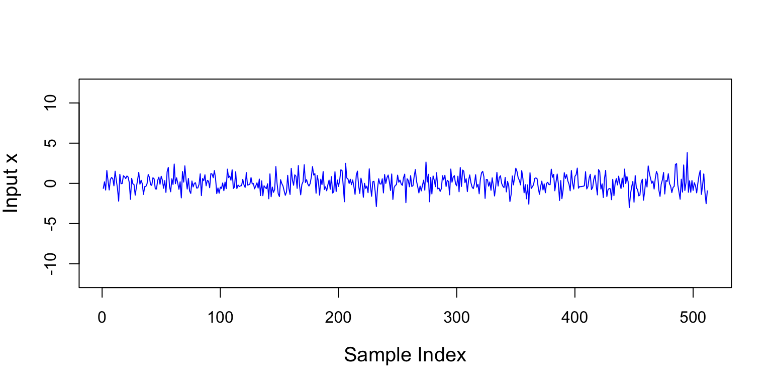
Below, we use the ARMA[1,1] model to produce simulated data. In this case, we let \(a[1] = 0.9\), \(b[1] = −0.9\), and the input \(x[n]\) is WGN with variance 1. The model specified above is written as \[ y[n] = −0.9y[n − 1] − 0.9x[n − 1] + x[n]. \tag{2}\]
Note the \(a[1]\) coefficient is 0.9. The negative sign in front of 0.9 is part of Equation 1. Below we use rnorm(N) to produce N samples of WGN with variance 1.
set.seed(1)
N <- 512
x <- rnorm(N)
Figure 1 is a plot of x, the input into the ARMA[1,1] process defined in Equation 2.
Below is the ARMA[1,1] model from Equation 2 implemented in R.
y_arma11 <- rep(0,N)
a <- 0.9
b <- -0.9
for (n in 2:N)
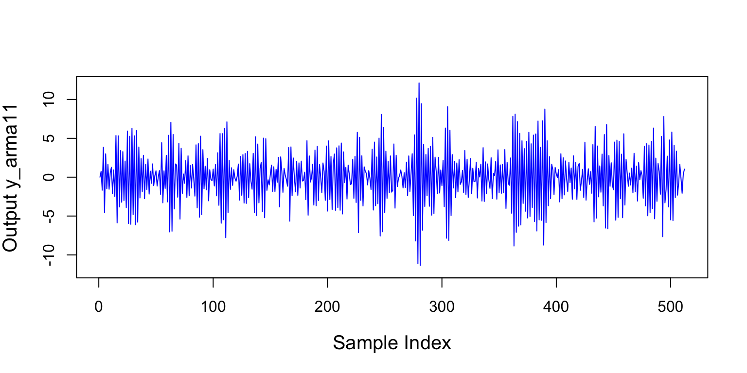
y_arma11[n] <- -a[1]*y_arma11[n-1]+ b[1]*x[n-1] + x[n] Figure 2 is a plot of y_arma11, the model’s output.
The PSD \(P(f)\) of an ARMA model is \[ P_{\text{ARMA}}(f) = \sigma^2 \left |\frac{ 1 + \sum_{k=1}^q b[k]\exp(-j2\pi fk) } { 1 + \sum_{k=1}^p a[k]\exp(-j2\pi fk) } \right |^2, \tag{3}\] where the \(a\)’s and \(b\)’s are the coefficients of the model and \(\sigma^2\) is the variance of the WGN input. Notice the numerator and denominator in Equation 3 are polynomials. The roots (zeros) of these polynomials control the shape of the PSD. The denominator’s roots are called poles, and they control the peaks (high parts). The numerator’s roots are called zeros and control the valleys (low parts). Note that the peaks are more important than the valleys in most (not all!) applications.
Because ARMA models have poles and zeros, they are good at modeling PSDs with peaks and valleys. When used for PSD estimation, ARMA estimators are called “high resolution” estimators because they are better than the periodogram at resolving closely spaced peaks.
If we let \[B(f) = 1 + \sum_{k=1}^q b[k]\exp(-j2\pi fk)\] and \[A(f) = 1 + \sum_{k=1}^p a[k]\exp(-j2\pi fk),\] then we can write Equation 3 as \[ P_{\text{ARMA}}(f) = \sigma^2 \left |\frac{B(f) } { A(f) } \right |^2 = \sigma^2 |B(f)|^2 \frac{1}{|A(f)|^2}. \tag{4}\] Notice \(A(f)\) is the Fourier transform of the \(a\)’s, and \(B(f)\) is the Fourier transform of the \(b\)’s. Equation 4 makes clear that the ARMA PSD is the product of the input variance \(\sigma^2\), \(|B(f)|^2\), and \(\frac{1}{|A(f)|^2}\). Note the PSD of white noise with variance \(\sigma^2\) is \(P_{\sigma^2}(f) = \sigma^2\), which is a constant.
The function psdArma inputs the ARMA parameters and output the PSD calculated at evenly spaced point along the frequency axis. The function inputs: the AR coefficients arCoefficients, the MA coefficients maCoefficients, the variance of the input process inputVar, and the number of points in the fft used to calculate the PSD. The function uses the fft function to find \(A(f)\) and \(B(f)\) in Equation 4. The function uses zeroPad (see below) to zero pad the AR and MA coefficients to produce Nfs frequency samples. The parameters must be known or estimated before using psdArma. If the parameters are known, the function outputs the PSD. If the parameters are estimated, the function outputs an estimated PSD.
zeroPad <- function(x,N) {
  c(x,rep(0,max(N-length(x),0)))
}
psdArma <- function(arCoefficients,maCoefficients,inputVar,Nfs=256){
A <- fft(zeroPad(arCoefficients,Nfs))
B <- fft(zeroPad(maCoefficients,Nfs))
inputVar*abs(B)^2/abs(A)^2
}Let’s use psdArma to calculate the PSD of the ARMA[1,1] process in Equation 2.
psdArma11 <- 10*log10(psdArma(c(1,a),c(1,b),inputVar=1,Nfs=length(x)))Figure 3 contains two plots. The blue plot is the PSD of the ARMA[1,1] process that produced the data in Figure 2. The black plot is the PSD of the WGN input.
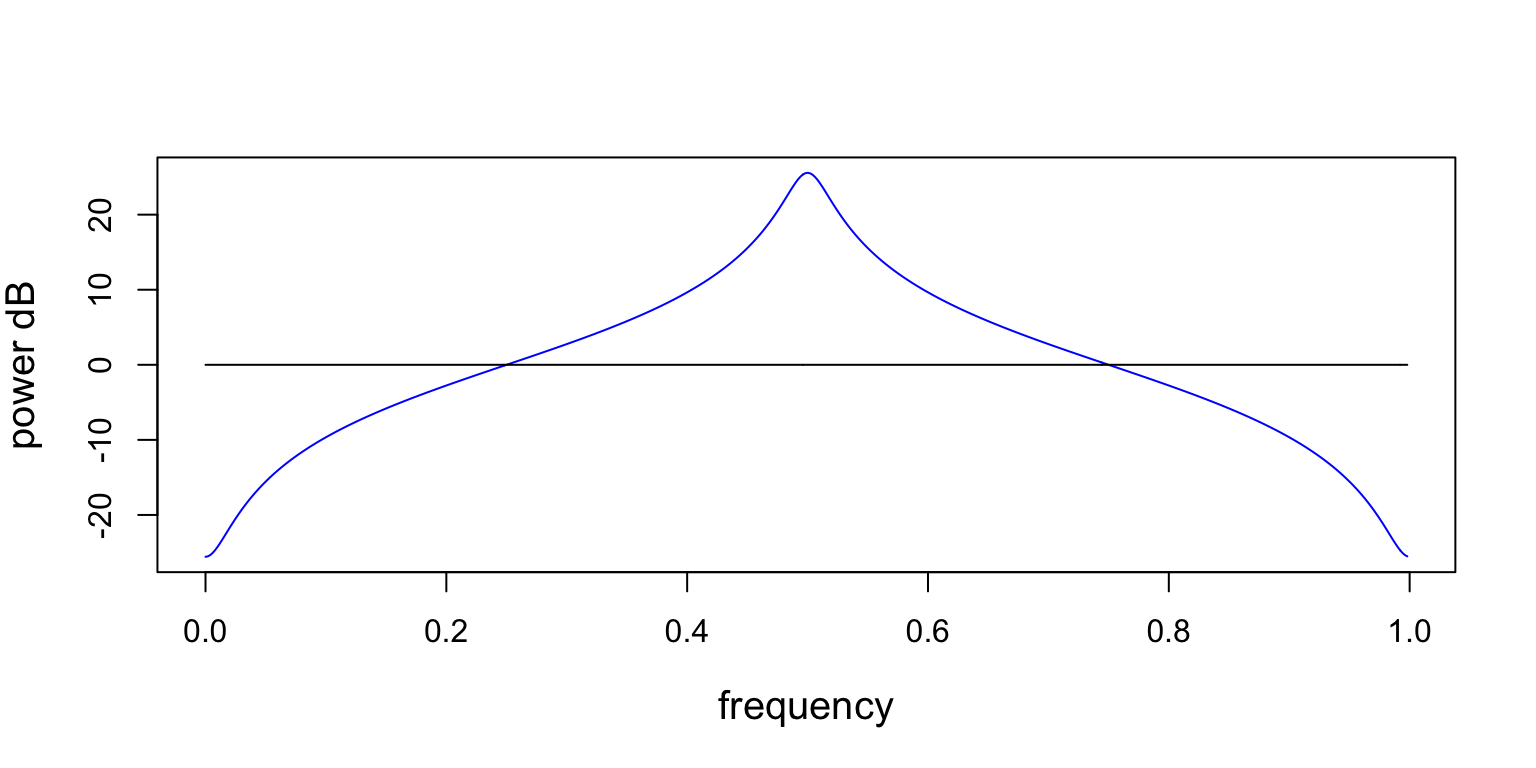
There are three things to notice about the PSD plots. First, the frequency units on the x-axis are a fraction of the sampling frequency (cycles/sample). If you know the sampling frequency (samples/second), you could recover frequency in Hz (cycles/second) by multiplying frequency by the sampling frequency, as \[ (\text{cycles/sample})(\text{samples/second})=(\text{cycles/second}).\]
Second, the y-axis is power in decibels (dB), calculated as \[\text{power dB} = 10\log_{10}(\text{power}).\]
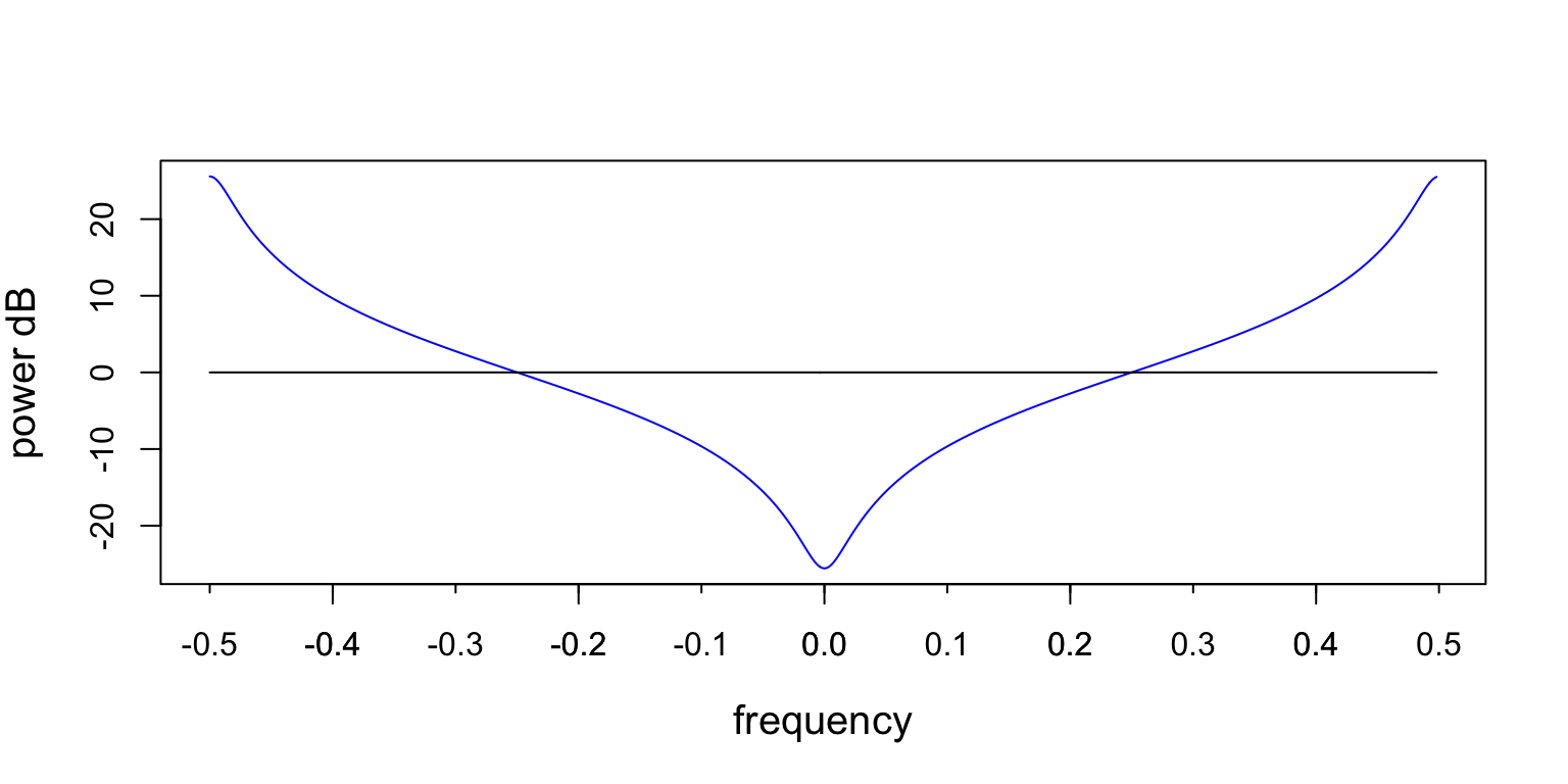
Third, PSDs are periodic with the sampling frequency. So, they can be plotted along any region that shows one period. Below is an example of the PSD from above plotted from -0.5 to 0.5.
3 Autoregresive Model
ARMA[\(p\),0] models are known as autoregressive (AR) models of order \(p\). The AR[\(p\)] model is written as \[ y[n] = -\sum_{k=1}^{p} a[k]y[n-k] + x[n], \tag{5}\] where the \(a[k]\)’s are the AR coefficients, \(x\) is the WGN input, and \(p\) is the process’s order.
We use the AR[1] model below to produce simulated data. We let \(a[1]=0.9\), and the input \(x[n]\) is WGN with variance 1. The model is written as \[ y[n] = -0.9y[n-1] + x[n], \tag{6}\]
We use a for loop to implement the ARMA model. We could do the same thing for the AR model, but using the filter command from the gsignal is faster and makes the code more readable. The function inputs the AR coefficients a, the MA coefficients b, and the samples to be filtered x. The function outputs the data filtered by the ARMA coefficients.
Figure 5 is a plot of the samples produced by the code below.
set.seed(1)
N <- 512
x <- rnorm(N)
a <- c(1.0, 0.9)
b <- 1
y_ar1 <- gsignal::filter(b,a,x)
The PSD of an AR process is \[ P_{\text{AR}}(f) = \frac{\sigma^2 } {|1 + \sum_{k=1}^p a[k]\exp(-j2\pi fk)|^2 }. \tag{7}\] Since Equation 7 has no zeros in the numerator; the AR PSD only has poles. The poles make AR models good at modeling PSDs with peaks. AR PSD estimators are high resolution estimators because they are good at resolving closely spaced peaks. AR models are good at modeling peaks and are simpler than ARMA models, so they are used more often than the other two.
Below we find the PSD of the AR[1] model above.
psdAr1 <- 10*log10(psdArma(a,b,inputVar=1,Nfs=length(x)))Figure 5 contains two plots. The blue plot is the PSD of the AR[1] process that produced the data in Figure 5. The black plot is the PSD of the WGN input.
psdAr1 <- 10*log10(psdArma(a,b,inputVar=1,Nfs=length(x)))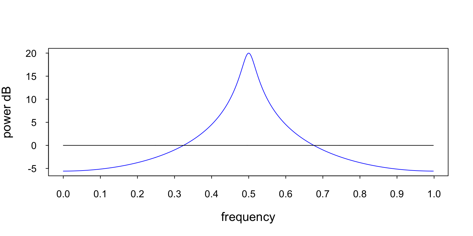
4 Moving Average Model
ARMA[0,\(q\)] models are known as moving average (MA) model of order \(q\). An MA[\(q\)] is written as \[ y[n] = \sum_{k=0}^q b[k]x[n-k], \tag{8}\] where the \(b[k]\)’s are the MA coefficients, \(x[k]\) is WGN input, and the \(q\) is the process’s order. The simple averaging filter is a special case of the MA model, where the MA parameters are \(\frac{1}{q+1}\). The simple averaging filter is written as \[ y[n] = \frac{1}{q+1}\sum_{k=0}^q x[n-k]. \] Below we use the MA[1] model to produce simulated data. We let \(b[1]=-0.9\), and the input \(x[n]\) is WGN with variance 1. The model is written as \[ y[n] = -0.9x[n-1] + x[n], \tag{9}\] Now we filter the complex WGN samples.
set.seed(1)
N <- 512
x <- rnorm(N)
a <- 1
b <- c(1,-0.9)
y_ma1 <- gsignal::filter(b,a,x)
Figure 7 is a plot of the samples produced by the code above.
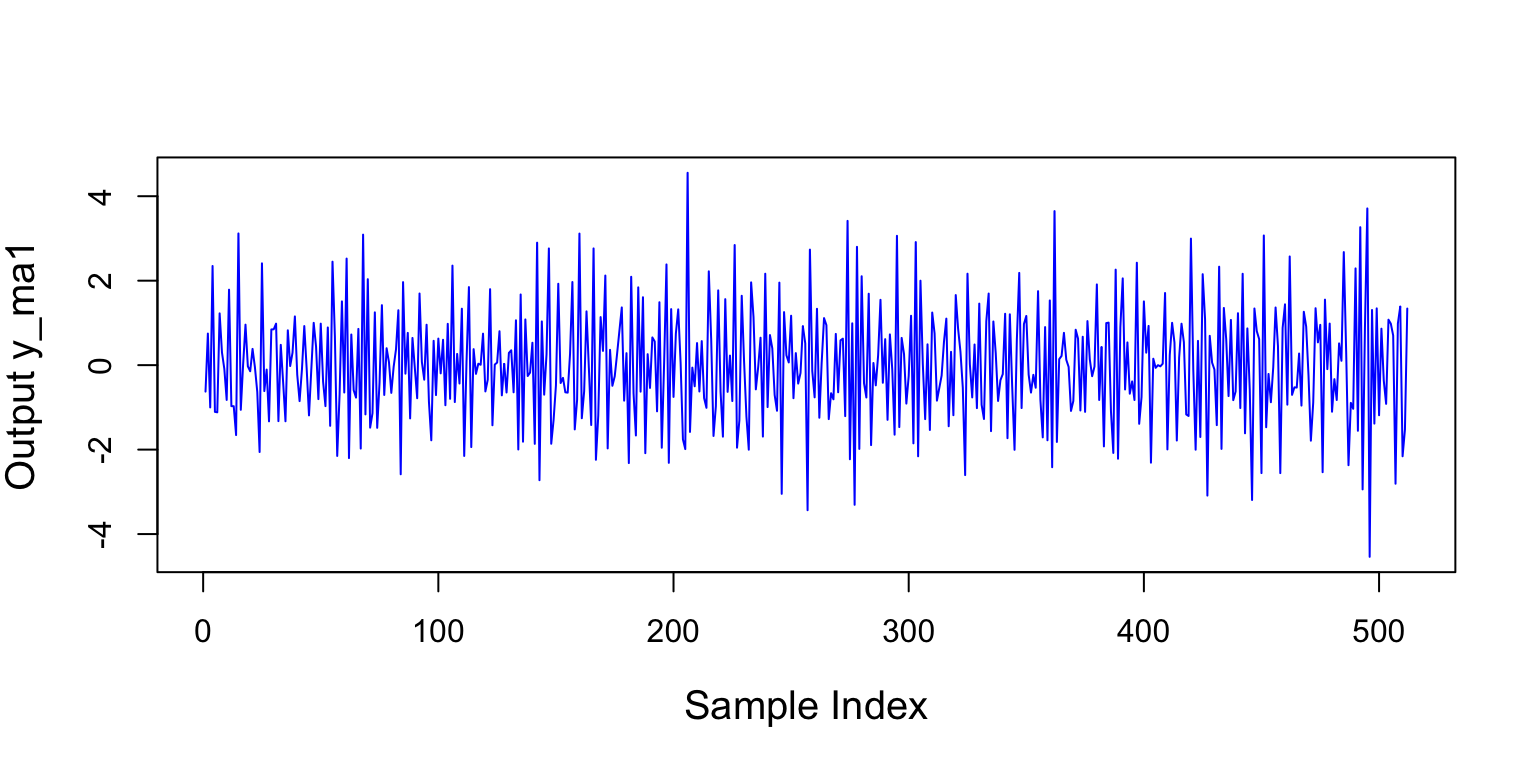
The PSD of an MA process is \[ P_{\text{MA}}(f) = \sigma^2 |1 + \sum_{k=1}^q b[k]\exp(-j2\pi fk)|^2. \tag{10}\] The MA PSD has zeros, but no poles. So, the MA model is good at modeling PSDs with deep valleys. The MA PSD estimator is not able to resolve closely spaced peaks.
Below we find the PSD of the MA[1] model above.
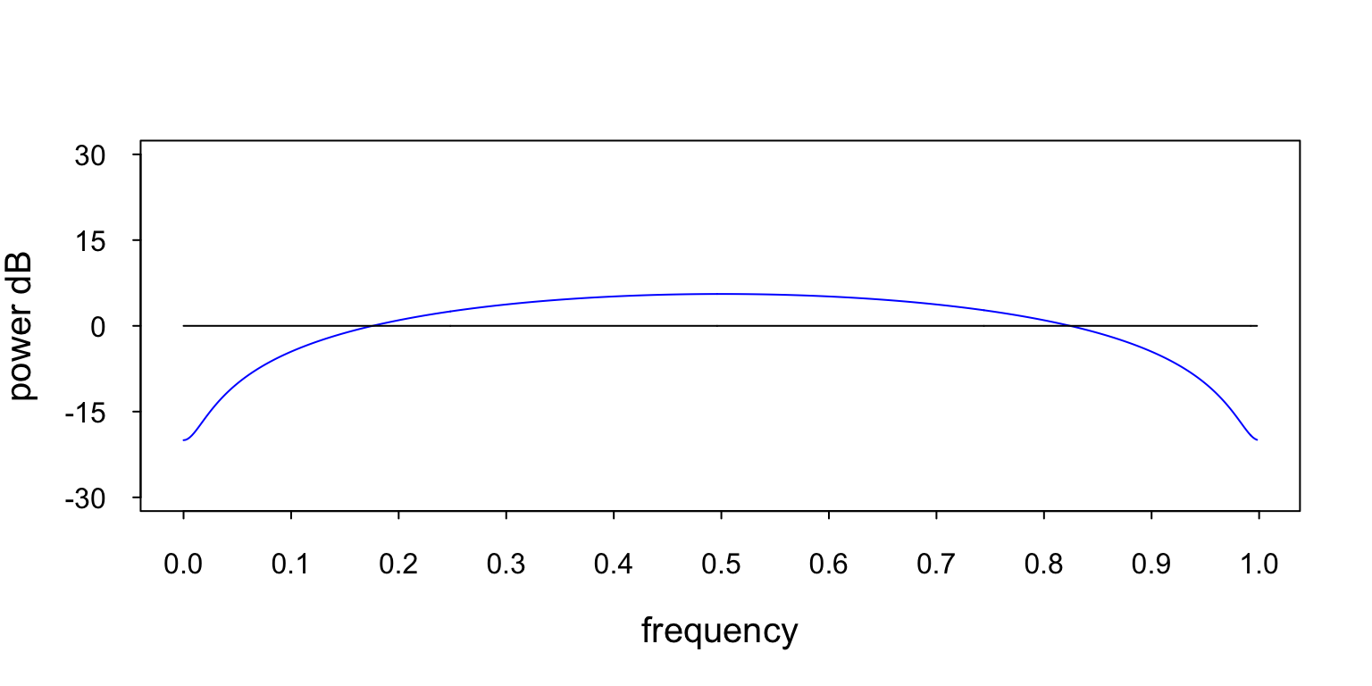
psdMa1 <- 10*log10(psdArma(a,b,inputVar=1,Nfs=length(x)))Figure 8 contains two plots. The blue plot is the PSD of the MA[1] process that produced the data in Figure 7. The black plot is the PSD of the WGN input.
5 Estimating PSDs using Models
ARMA/AR/MA PSD estimation is performed using the following steps. First, choose the model you wish to use. Second, use the data to estimate the model parameters. Parameter estimation is beyond the scope of this article. You can find information in various places, including Carbone (2022), Kay (1988), or Marple (1987). Finally, calculate the estimated PSD using the estimated parameters in the psdArma function.
6 Choosing a Model
If you are only interested in peaks, use the AR model. If only the valleys are important, use the MA model. If both the peaks and valleys are important, use the ARMA model. As mentioned above, peaks are usually the more important feature, so the AR model is often chosen.
7 Model Order Selection
An ARMA model can model at most \(p\) peaks and \(q\) nulls. So, if you know the number of peaks and valleys in the PSD, choosing the model order is straightforward. For instance, if the PSD had one peak and two nulls, you would use an ARMA[1,2] model. Unfortunately, we don’t always know the number of peaks and nulls, but we can use a model order estimator to help us choose the model order.
Model order estimators are mathematical tools that let you estimate the order of the process that produced the data. The Akaike Information Criterion (AIC) is a model order estimator built into the arima function. The AIC calculates how well the model fits the data (lower is better).
The arima function produces several outputs, but we will use the AIC. So we use the arima function with $aic, which will only output the AIC value. The arima$aic function inputs the data and the model order and then outputs the AIC associated with that model order. Below is an example of using the function to find the model order.
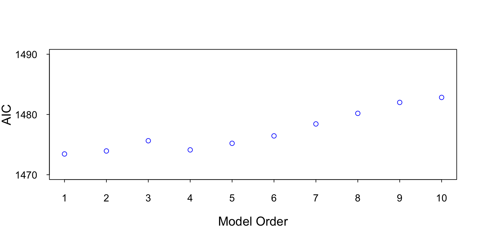
Below we use the AR[1] data shown in Figure 5 and calculate the AIC for AR model orders 1 to 10.
aicAR <- rep(0,10)
for (modelOrder in 1:10) {
  aicAR[modelOrder] <- arima(y_ar1, order = c(AR=modelOrder, 0, MA=0))$aic
}
Figure 9 is a plot of the AIC for AR models 1 to 10. Note the minimum AIC is at AR[1], which is the correct model order.
However, we choose the model order; we don’t want to overfit the model. We want to choose the minimum model order that can model the important features. Overfitting the model requires more parameters and can add bias and variance to our estimate.


No comments:
Post a Comment